mvabund
mvabund.RmdThis vignette takes you through the main functions in mvabund to help you get started! We recommend reading the manuscript associated with the package and taking a look at Other Resources in our README.
First things first
Let’s load the package and get our hands on the Tasmania data set to look at the effects of disturbance treatment on invertebrate abundances. Note that the Tasmania data set is a list object. We will only look at the copepods data frame for this walk-through. The copepods data frame can be accessed using Tasmania$copepods or the attach() function which will make the contents of Tasmania searchable.
Visualise the multivariate data
We first need to turn our data into a mvabund object so functions for this package and work with the data
copepod_abund <- mvabund(copepods)Now lets take a look at abundance for each species across our treatment sites (Disturbed vs. Undisturbed). Observations were collected using a spatially blocked design where researchers took four samples at each block (2 per treatment). We can set the colour (col) of the points to represent that four sampling blocks
plot(copepod_abund~treatment, col = block)
#> Overlapping points were shifted along the y-axis to make them visible.
#>
#>  PIPING TO 2nd MVFACTOR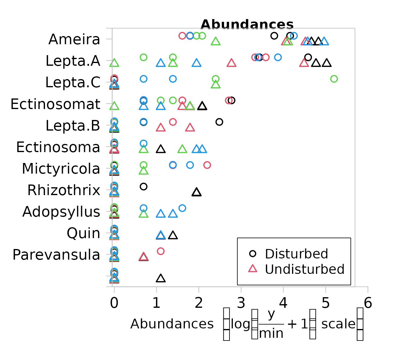
Fitting Predictive Models
It was hypothesised that the abundance of Ameira and Ectinosoma was reduced in Disturbed sites, whereas the abundance of Mictyricola may have increased. Lets test this hypothesis using the manyglm() function. This function fits a generalised linear model for each species. We specified family = "negative.binomial" as count data tends to follow a negative binomial distribution. Other distributions are available too! See ?manyglm()
cope.nb <- manyglm(copepods ~ treatment*block, family = "negative.binomial")Checking Model Assumptions
Before we look at the model output, we should check on the model residuals. What we want to see is little pattern as this implies that our choice of negative binomial distribution is appropriate.
plot(cope.nb)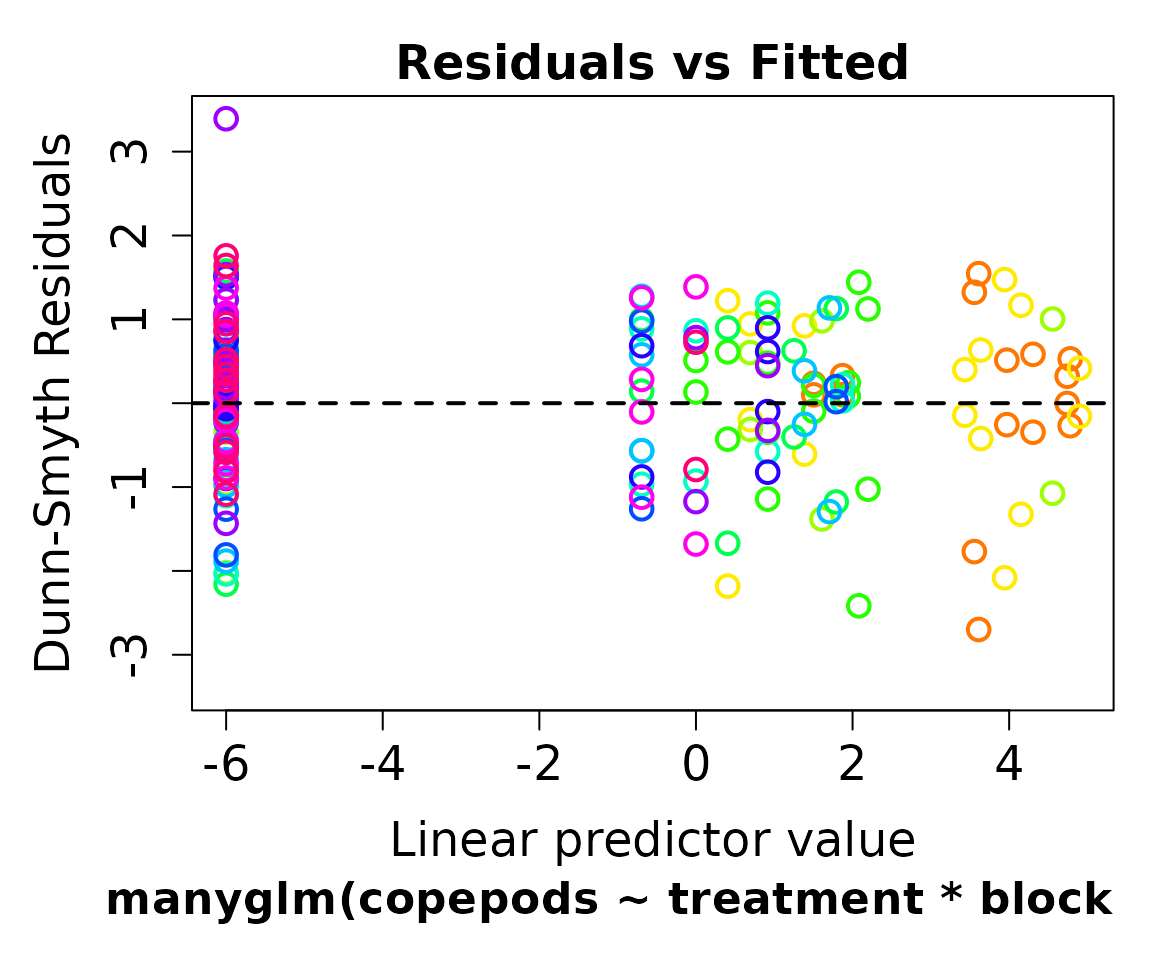
Now, lets proceed to check on the mean-variance relationship. We want to to see if the mean-variance relationship of our data adheres to that of a negative binomial distribution which tends to be quadratic rather than linear. The meanvar.plot() function plots the sample variance against the sample mean for each species within each factor level of (tr.block). A quadratic relationship seems appropriate for our sample mean and variance.
meanvar.plot(copepods~tr.block, col = treatment)
#> START SECTION 2
#> Plotting if overlay is TRUE
#> using grouping variable tr.block 46 mean values were 0 and could
#>                                      not be included in the log-plot
#> using grouping variable tr.block 49 variance values were 0 and could not
#>                                      be included in the log-plot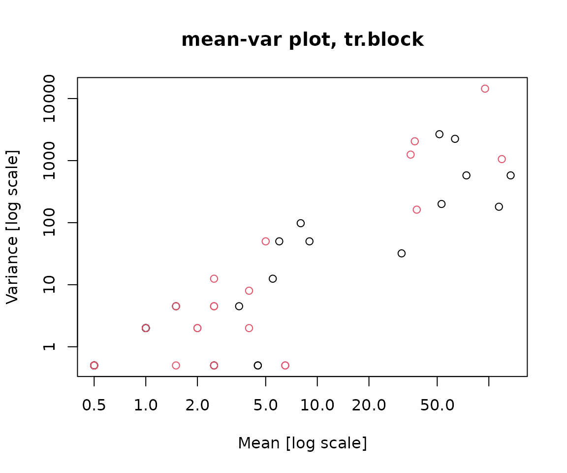
#> FINISHED SECTION 2Hypothesis Testing
To test whether treatment and block had an effect on the abundances of copepods we can use the anova() function. This function returns a Analysis of Deviance table which tests the significance of each model term. Setting p.uni = "adjusted" allows for our p-values to be adjusted for multiple testing of different species.
anova(cope.nb, p.uni = "adjusted")
#> Time elapsed: 0 hr 0 min 9 sec
#> Analysis of Deviance Table
#>
#> Model: copepods ~ treatment * block
#>
#> Multivariate test:
#>                 Res.Df Df.diff    Dev Pr(>Dev)
#> (Intercept)         15
#> treatment           14       1  32.52    0.056 .
#> block               11       3 151.87    0.001 ***
#> treatment:block      8       3  37.41    0.083 .
#> ---
#> Signif. codes:  0 '***' 0.001 '**' 0.01 '*' 0.05 '.' 0.1 ' ' 1
#>
#> Univariate Tests:
#>                 Ameira          Adopsyllus          Ectinosoma
#>                    Dev Pr(>Dev)        Dev Pr(>Dev)        Dev Pr(>Dev)
#> (Intercept)
#> treatment        6.257    0.166      0.032    0.972      7.026    0.151
#> block           12.615    0.154     17.691    0.049     15.361    0.069
#> treatment:block  6.349    0.498      1.295    0.899      0.836    0.902
#>                 Ectinosomat          Haloschizo          Lepta.A
#>                         Dev Pr(>Dev)        Dev Pr(>Dev)     Dev Pr(>Dev)
#> (Intercept)
#> treatment             0.366    0.952      1.497    0.830   0.281    0.952
#> block                 10.92    0.179      3.742    0.269  20.756    0.015
#> treatment:block       1.122    0.902          0    0.902  13.072    0.179
#>                 Lepta.B          Lepta.C          Mictyricola
#>                     Dev Pr(>Dev)     Dev Pr(>Dev)         Dev Pr(>Dev)
#> (Intercept)
#> treatment         0.575    0.952   2.141    0.761       7.093    0.151
#> block               8.8    0.179  17.419    0.049      11.415    0.179
#> treatment:block   7.402    0.436    0.34    0.902       5.268    0.498
#>                 Parevansula           Quin          Rhizothrix
#>                         Dev Pr(>Dev)   Dev Pr(>Dev)        Dev Pr(>Dev)
#> (Intercept)
#> treatment                 0    0.988 5.385    0.208      1.869    0.761
#> block                   6.1    0.179  9.44    0.179     17.613    0.049
#> treatment:block       1.726    0.872     0    0.902          0    0.902
#> Arguments:
#>  Test statistics calculated assuming uncorrelated response (for faster computation)
#> P-value calculated using 999 iterations via PIT-trap resampling.
We can see that there is a significant effect of the treatment factor meaning that treatment has a significant multiplicative effect on mean abundance. The interaction between blocks and treatments is not significant, meaning that the multiplicative treatment effect is consistent across blocks.
If you do not have a specific hypothesis in mind that you want to test, and are instead interested in which model terms are statistically significant, then the summary() function will come in handy. However results aren’t quite as trustworthy as for anova(). The reason is that re-samples are taken under the alternative hypothesis for summary(), where there is a greater chance of fitted values being zero, especially for rarer taxa (e.g. if there is a treatment combination in which a taxon is never present). Abundances don’t re-sample well if their predicted mean is zero.
summary(cope.nb)
#>
#> Test statistics:
#>                             wald value Pr(>wald)
#> (Intercept)                     18.493     0.001 ***
#> treatmentUndisturbed             3.330     0.240
#> block2                           4.710     0.038 *
#> block3                           6.650     0.001 ***
#> block4                           3.435     0.144
#> treatmentUndisturbed:block2      2.747     0.259
#> treatmentUndisturbed:block3      1.615     0.443
#> treatmentUndisturbed:block4      4.262     0.050 *
#> ---
#> Signif. codes:  0 '***' 0.001 '**' 0.01 '*' 0.05 '.' 0.1 ' ' 1
#>
#> Test statistic:  14.81, p-value: 0.004
#> Arguments:
#>  Test statistics calculated assuming response assumed to be uncorrelated
#>  P-value calculated using 999 resampling iterations via pit.trap resampling (to account for correlation in testing).
If obtaining predicted values from the model is the goal, you may use the predict() function. Note that type = response will produce values on the scale of the response variable (i.e. counts)
predict(cope.nb, type = "response")
#>      Ameira   Adopsyllus   Ectinosoma Ectinosomat   Haloschizo Lepta.A
#> B1D1   53.0 3.678795e-07 3.678794e-07         8.0 3.678794e-07    63.5
#> B1D2   53.0 3.678795e-07 3.678794e-07         8.0 3.678794e-07    63.5
#> B1U1  114.5 3.678794e-07 1.000000e+00         7.0 1.000000e+00   134.0
#> B1U2  114.5 3.678794e-07 1.000000e+00         7.0 1.000000e+00   134.0
#> B2D1    4.5 3.678794e-07 3.678794e-07         9.0 3.678794e-07    31.0
#> B2D2    4.5 3.678794e-07 3.678794e-07         9.0 3.678794e-07    31.0
#> B2U1   74.0 3.678794e-07 3.678794e-07         4.5 3.678794e-07    51.5
#> B2U2   74.0 3.678794e-07 3.678794e-07         4.5 3.678794e-07    51.5
#> B3D1    6.5 3.678794e-07 3.678794e-07         2.5 3.678794e-07     2.0
#> B3D2    6.5 3.678794e-07 3.678794e-07         2.5 3.678794e-07     2.0
#> B3U1   35.0 5.000000e-01 2.500000e+00         2.5 3.678794e-07     1.5
#> B3U2   35.0 5.000000e-01 2.500000e+00         2.5 3.678794e-07     1.5
#> B4D1   37.0 2.500000e+00 5.000000e-01         1.0 3.678794e-07    38.0
#> B4D2   37.0 2.500000e+00 5.000000e-01         1.0 3.678794e-07    38.0
#> B4U1  119.0 2.500000e+00 6.500000e+00         1.5 3.678794e-07     4.0
#> B4U2  119.0 2.500000e+00 6.500000e+00         1.5 3.678794e-07     4.0
#>           Lepta.B      Lepta.C  Mictyricola  Parevansula         Quin
#> B1D1 6.000000e+00 3.678794e-07 3.678795e-07 3.678794e-07 3.678794e-07
#> B1D2 6.000000e+00 3.678794e-07 3.678795e-07 3.678794e-07 3.678794e-07
#> B1U1 3.678794e-07 3.678794e-07 3.678794e-07 5.000000e-01 2.500000e+00
#> B1U2 3.678794e-07 3.678794e-07 3.678794e-07 5.000000e-01 2.500000e+00
#> B2D1 1.500000e+00 3.678794e-07 5.500000e+00 1.000000e+00 3.678794e-07
#> B2D2 1.500000e+00 3.678794e-07 5.500000e+00 1.000000e+00 3.678794e-07
#> B2U1 3.500000e+00 3.678794e-07 3.678794e-07 5.000000e-01 3.678794e-07
#> B2U2 3.500000e+00 3.678794e-07 3.678794e-07 5.000000e-01 3.678794e-07
#> B3D1 3.678794e-07 9.500000e+01 5.000000e-01 3.678794e-07 3.678794e-07
#> B3D2 3.678794e-07 9.500000e+01 5.000000e-01 3.678794e-07 3.678794e-07
#> B3U1 3.678794e-07 5.000000e+00 5.000000e-01 3.678794e-07 3.678794e-07
#> B3U2 3.678794e-07 5.000000e+00 5.000000e-01 3.678794e-07 3.678794e-07
#> B4D1 5.000000e-01 2.000000e+00 4.000000e+00 3.678794e-07 3.678794e-07
#> B4D2 5.000000e-01 2.000000e+00 4.000000e+00 3.678794e-07 3.678794e-07
#> B4U1 3.678794e-07 3.678794e-07 3.678794e-07 3.678794e-07 1.000000e+00
#> B4U2 3.678794e-07 3.678794e-07 3.678794e-07 3.678794e-07 1.000000e+00
#>        Rhizothrix
#> B1D1 5.000000e-01
#> B1D2 5.000000e-01
#> B1U1 6.000000e+00
#> B1U2 6.000000e+00
#> B2D1 3.678794e-07
#> B2D2 3.678794e-07
#> B2U1 3.678794e-07
#> B2U2 3.678794e-07
#> B3D1 3.678794e-07
#> B3D2 3.678794e-07
#> B3U1 3.678794e-07
#> B3U2 3.678794e-07
#> B4D1 3.678794e-07
#> B4D2 3.678794e-07
#> B4U1 3.678794e-07
#> B4U2 3.678794e-07