Chapter 2 -- An importance equivalence result -- Exercise solutions and Code Boxes

Exercise 2.1 Two-sample t-test for guinea pig experiment

See Code Box 2.1, \(P\)-value is about 0.008. This means that the test statistic is unusually small so there is good evidence of an effect of nicotine. More directly, starting from the stated test statistic of \(-2.67\), the test statistic has a \(t_{n_1+n_2-2}\) distribution under the hypothesis of no effect, so we could calculate the \(P\)-value directly as:

 pt(-2.67,10+10-2)
#> [1] 0.007807045

Code Box 2.1 A two-sample t-test of the data from the guinea pig experiment

 library(ecostats)
#> Loading required package: mvabund
 data(guineapig)
 t.test(errors~treatment, data=guineapig, var.equal=TRUE, alternative="less")
#> 
#>  Two Sample t-test
#> 
#> data:  errors by treatment
#> t = -2.671, df = 18, p-value = 0.007791
#> alternative hypothesis: true difference in means between group C and group N is less than 0
#> 95 percent confidence interval:
#>       -Inf -7.331268
#> sample estimates:
#> mean in group C mean in group N 
#>            23.4            44.3

Code Box 2.2: Smoking and pregnancy – checking assumptions

The normal quantile plots of Figure 2.1 were generated using the below code.

qqenvelope(guineapig$errors[guineapig$treatment=="N"])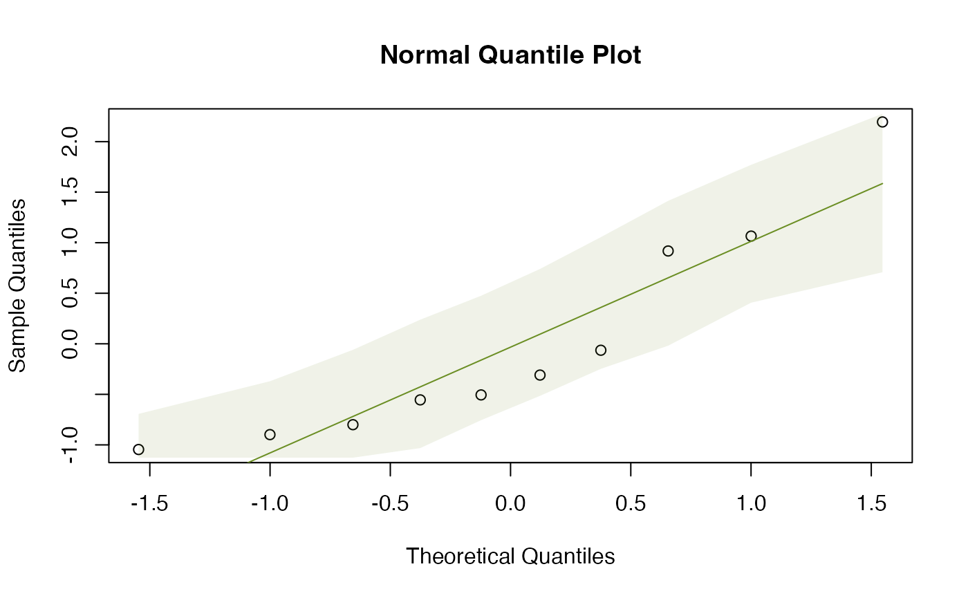

qqenvelope(guineapig$errors[guineapig$treatment=="C"])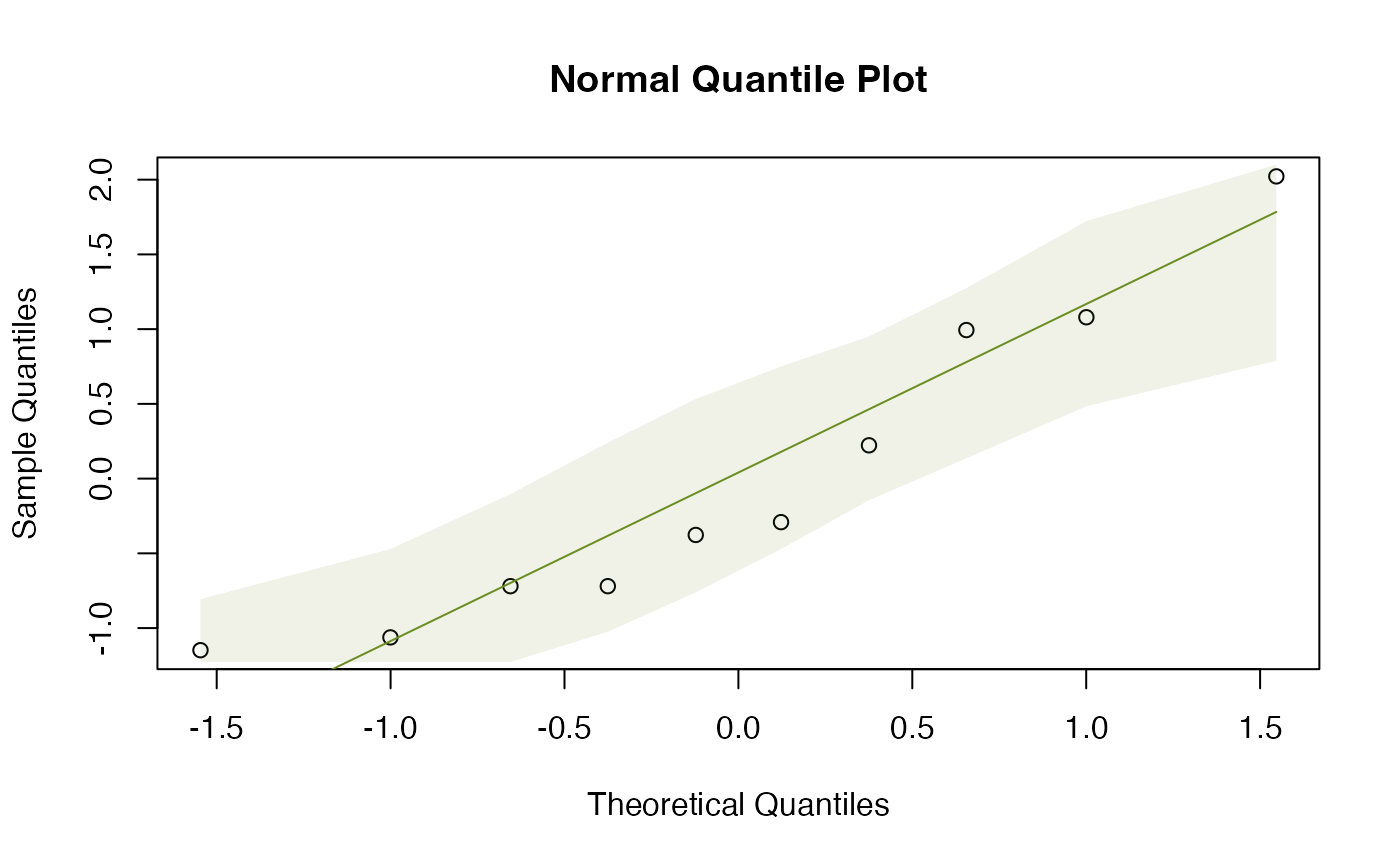

by(guineapig$errors,guineapig$treatment,sd)
#> guineapig$treatment: C
#> [1] 12.30357
#> ------------------------------------------------------------ 
#> guineapig$treatment: N
#> [1] 21.46858

While all the points lie in the simulation envelope, there is a clear curve on both of them suggesting some right skew. Also, the standard deviations are quite different, not quite a factor of two, but getting close. So it might be worth looking at (log-)transformation.

Exercise 2.2: Water quality

The research question is how it [IBI] related to catchment area which is an estimation question, we want to estimate the relationship between IBI and catchment area.

There are two variables:

catchment area is quantitative
Water quality (IBI) is quantitative

I would use a scatterplot:

 data(waterQuality)
 plot(quality~logCatchment, data=waterQuality)

And I would fit a linear regression model, as in Code Box 2.3.

Code Box 2.3: Fitting a linear regression to the water quality data

 data(waterQuality)
 fit_qual=lm(quality~logCatchment, data = waterQuality)
 summary(fit_qual)
#> 
#> Call:
#> lm(formula = quality ~ logCatchment, data = waterQuality)
#> 
#> Residuals:
#>    Min     1Q Median     3Q    Max 
#> -7.891 -3.354 -1.406  4.102 11.588 
#> 
#> Coefficients:
#>              Estimate Std. Error t value Pr(>|t|)    
#> (Intercept)    74.266      7.071  10.502 1.38e-08 ***
#> logCatchment  -11.042      1.780  -6.204 1.26e-05 ***
#> ---
#> Signif. codes:  0 '***' 0.001 '**' 0.01 '*' 0.05 '.' 0.1 ' ' 1
#> 
#> Residual standard error: 5.397 on 16 degrees of freedom
#> Multiple R-squared:  0.7064, Adjusted R-squared:  0.688 
#> F-statistic: 38.49 on 1 and 16 DF,  p-value: 1.263e-05

Exercise 2.3: Water quality – interpreting R output

An approximate 95% CI is

 -11.042+c(-2,2)*1.780
#> [1] -14.602  -7.482

or you could use confint:

 confint(fit_qual)
#>                  2.5 %   97.5 %
#> (Intercept)   59.27480 89.25623
#> logCatchment -14.81464 -7.26864

Either way we are 95% confident that as logCatchment changes by 1 (meaning a ten-fold increase in catchment area, since a log10-transformed of catchment area was used), IBI decreases by between about 7 and 15.

Code Box 2.4: Diagnostic plots for the water quality data

To produce a residual vs fits plot, and a normal quantile plot of residuals, you just take a fitted regression object (like fit_qual, produced in Code Box 2.3) and apply the plot function:

 plot(fit_qual, which=1:2)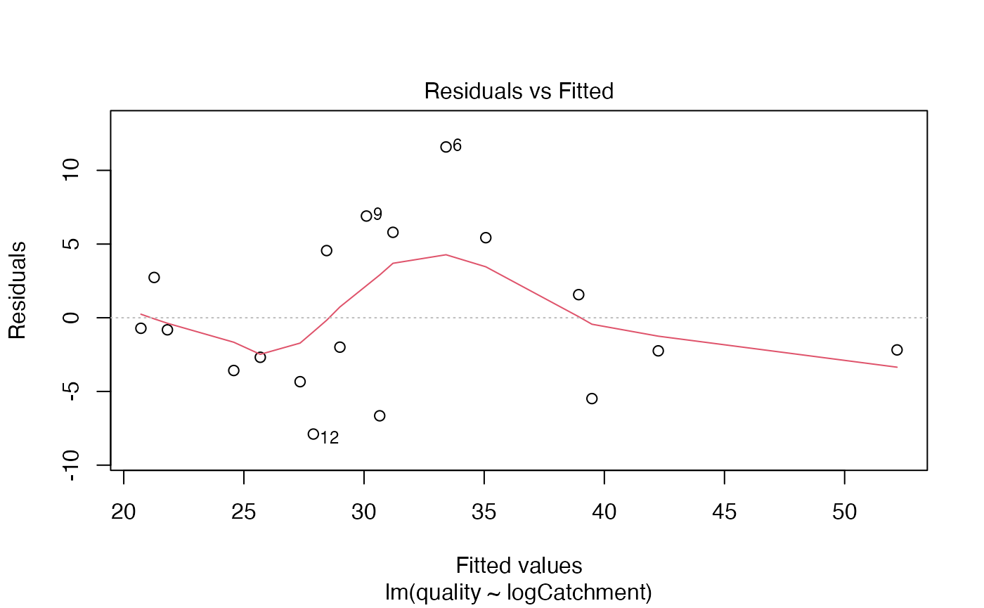

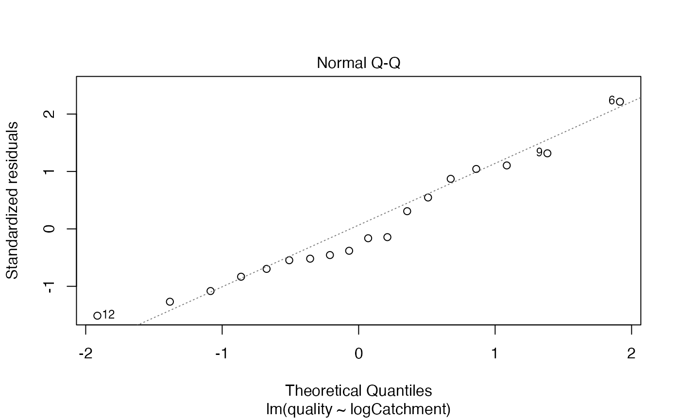
The which argument lets you choose which plot to construct (1=residuals vs fits, 2=normal quantile plot).

Alternatively, we can use ecostats::plotenvelope to add simulation envelopes around points on these plots, to check if any deviations from expected patterns are large compared to what we might expect for datasets that satisfy model assumptions:

 library(ecostats)
 plotenvelope(fit_qual, which=1:2)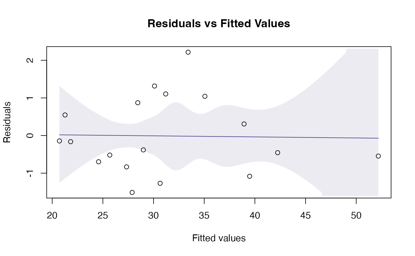

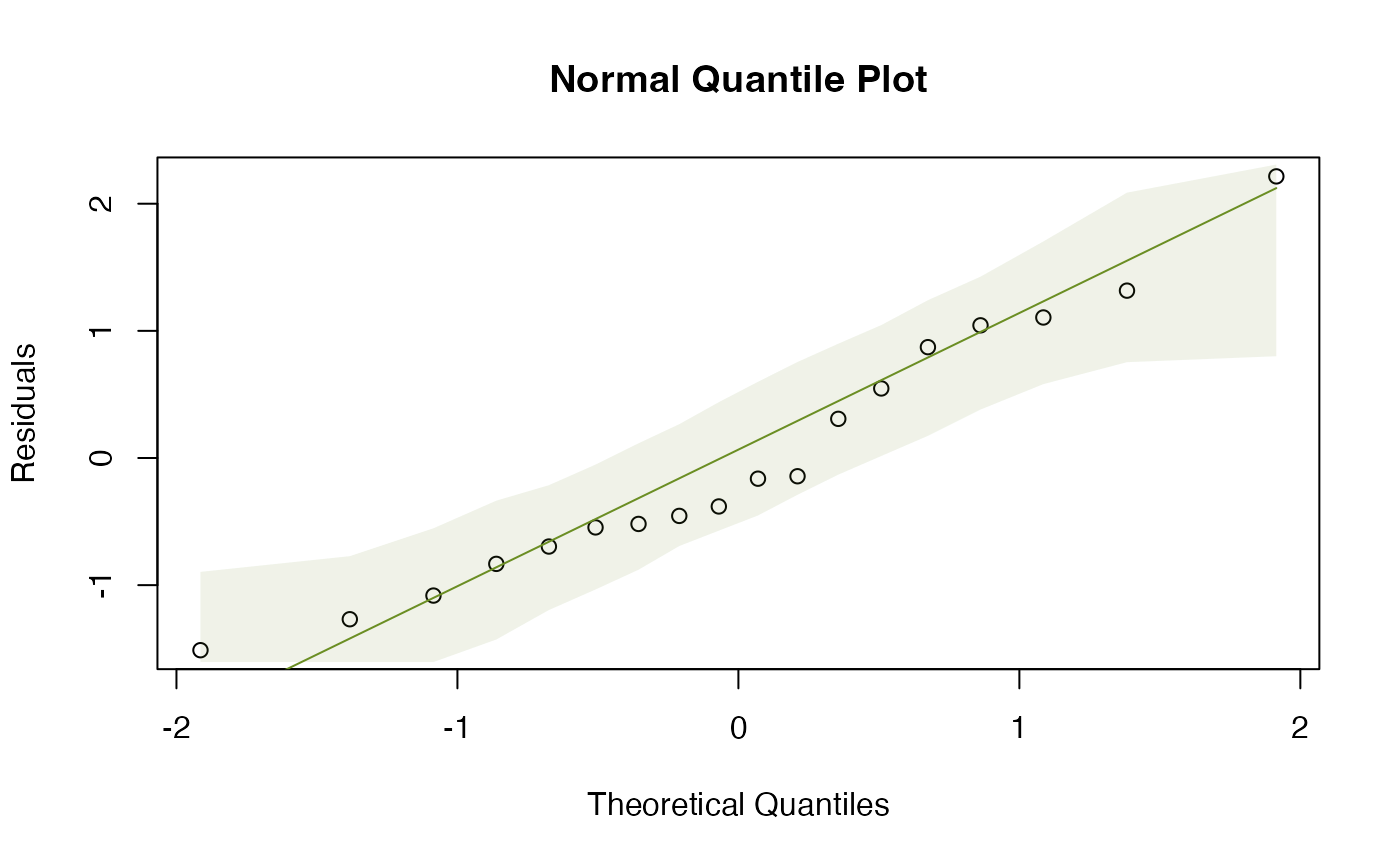
Assumptions look reasonable here – there is no trend in the residual vs fits plot, and the normal quantile plot is close to a straight line. Points are all well within their simulation envelopes, suggesting that departures are also small compared to what would be expected if the model were correct.

Exercise 2.4: Water quality{ assumption checks

There are four regression assumptions:

(conditional) independence: this cannot be checked using these plots, and depends primarily on the study design
Normality can be checked using the normal quantile plot of residuals, and it looks pretty good here.
Equal variance can be checked by looking for a fan shape in the residual vs fits plot, and there is no such trend here.
Linearity can be checked by looking for a U-shape in the residual vs fits plot, and there is no pattern so there are no concerns about this assumption here.

Code Box 2.5: Two-sample t-test output for the smoking-pregnant data, again

 t.test(errors~treatment, data=guineapig, var.equal=TRUE)
#> 
#>  Two Sample t-test
#> 
#> data:  errors by treatment
#> t = -2.671, df = 18, p-value = 0.01558
#> alternative hypothesis: true difference in means between group C and group N is not equal to 0
#> 95 percent confidence interval:
#>  -37.339333  -4.460667
#> sample estimates:
#> mean in group C mean in group N 
#>            23.4            44.3

Code Box 2.6: Linear regression analysis of the smoking-pregnant data. compare to Code Box 2.5

 ft_guineapig=lm(errors~treatment,data=guineapig)
 summary(ft_guineapig)
#> 
#> Call:
#> lm(formula = errors ~ treatment, data = guineapig)
#> 
#> Residuals:
#>    Min     1Q Median     3Q    Max 
#> -21.30 -11.57  -5.35  11.85  44.70 
#> 
#> Coefficients:
#>             Estimate Std. Error t value Pr(>|t|)    
#> (Intercept)   23.400      5.533   4.229 0.000504 ***
#> treatmentN    20.900      7.825   2.671 0.015581 *  
#> ---
#> Signif. codes:  0 '***' 0.001 '**' 0.01 '*' 0.05 '.' 0.1 ' ' 1
#> 
#> Residual standard error: 17.5 on 18 degrees of freedom
#> Multiple R-squared:  0.2838, Adjusted R-squared:  0.2441 
#> F-statistic: 7.134 on 1 and 18 DF,  p-value: 0.01558

Exercise 2.5: Global plant height against latitude

Angela has two variables of interest – height and latitude – and both are quantitative. So linear regression is a good starting point.

 library(ecostats)
 data(globalPlants)
 plot(height~lat,data=globalPlants)

 ft_height=lm(height~lat,data=globalPlants)
 summary(ft_height)
#> 
#> Call:
#> lm(formula = height ~ lat, data = globalPlants)
#> 
#> Residuals:
#>     Min      1Q  Median      3Q     Max 
#> -15.740  -7.905  -5.289   4.409  68.326 
#> 
#> Coefficients:
#>             Estimate Std. Error t value Pr(>|t|)    
#> (Intercept) 17.00815    2.61957   6.493 1.66e-09 ***
#> lat         -0.20759    0.06818  -3.045  0.00282 ** 
#> ---
#> Signif. codes:  0 '***' 0.001 '**' 0.01 '*' 0.05 '.' 0.1 ' ' 1
#> 
#> Residual standard error: 13.59 on 129 degrees of freedom
#> Multiple R-squared:  0.06705,    Adjusted R-squared:  0.05982 
#> F-statistic: 9.271 on 1 and 129 DF,  p-value: 0.002823
 plotenvelope(ft_height,which=1:2)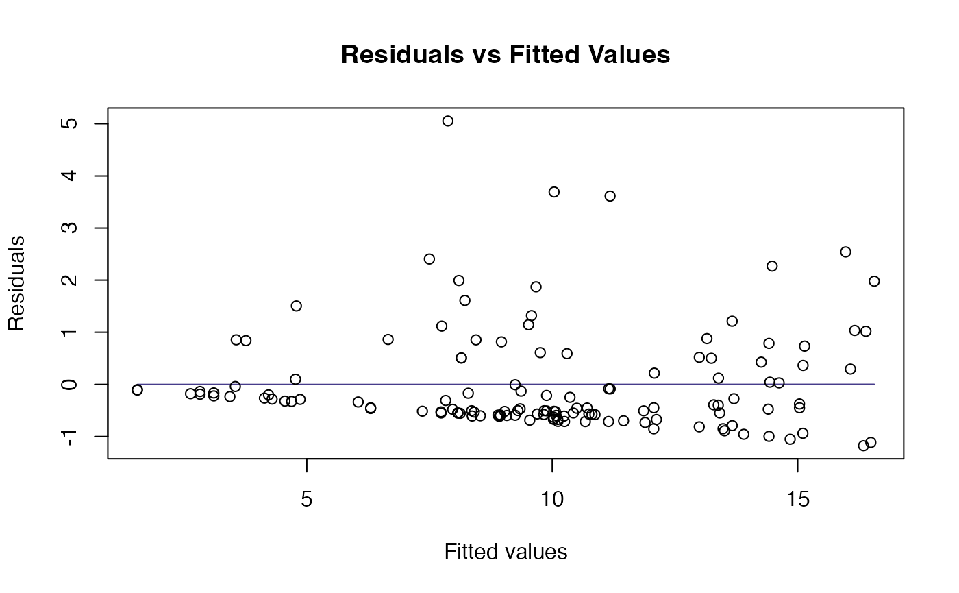

The original scatterplot suggests data are “pushed up” against the boundary of height=0, suggesting log-transformation. The linear model residual plots substantiate this, with the normal quantile plot clearly being strongly right-skewed, and the residual vs fits plot suggesting a fan-shape.

So let’s log-transform height.

 plot(height~lat,data=globalPlants,log="y")

 globalPlants$logHeight=log10(globalPlants$height) 
 ft_logHeight=lm(logHeight~lat,data=globalPlants)
 summary(ft_logHeight)
#> 
#> Call:
#> lm(formula = logHeight ~ lat, data = globalPlants)
#> 
#> Residuals:
#>      Min       1Q   Median       3Q      Max 
#> -1.49931 -0.48368 -0.04697  0.41125  1.54347 
#> 
#> Coefficients:
#>              Estimate Std. Error t value Pr(>|t|)    
#> (Intercept)  1.152525   0.124193   9.280 5.19e-16 ***
#> lat         -0.018501   0.003232  -5.724 6.94e-08 ***
#> ---
#> Signif. codes:  0 '***' 0.001 '**' 0.01 '*' 0.05 '.' 0.1 ' ' 1
#> 
#> Residual standard error: 0.6442 on 129 degrees of freedom
#> Multiple R-squared:  0.2025, Adjusted R-squared:  0.1963 
#> F-statistic: 32.76 on 1 and 129 DF,  p-value: 6.935e-08
 plotenvelope(ft_logHeight,which=1:2)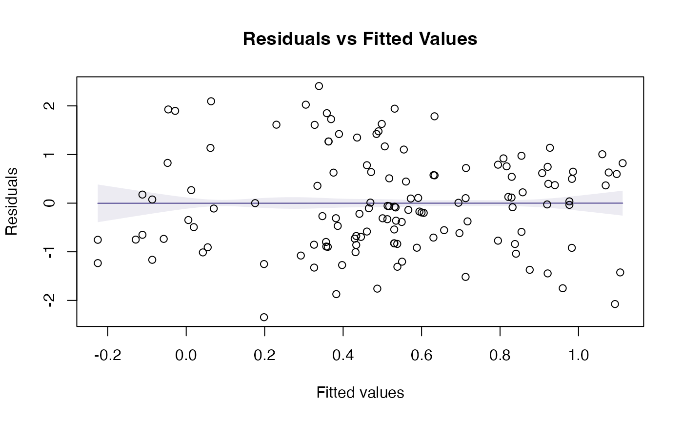

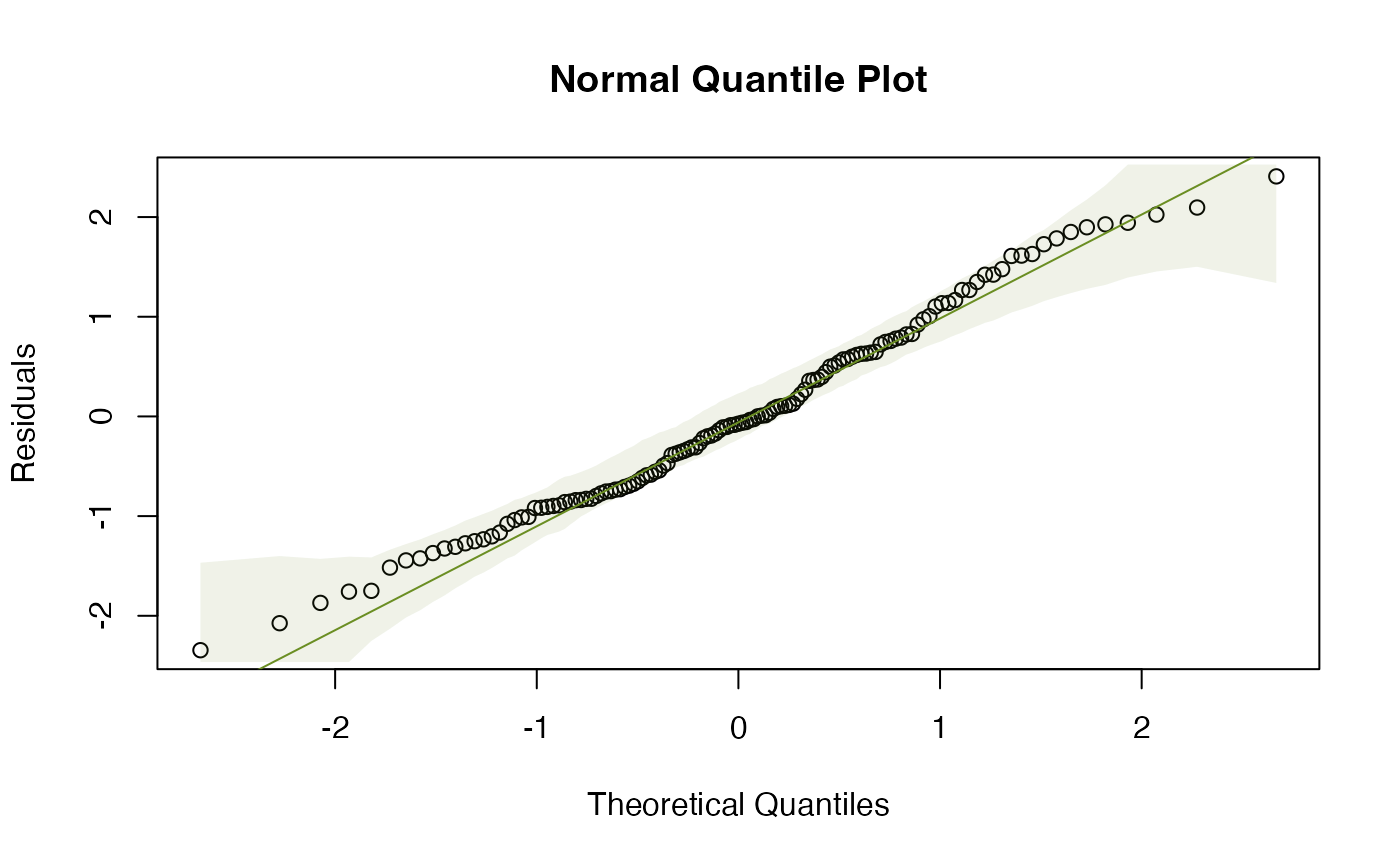
OK suddenly everything is looking a lot better!

Exercise 2.6: Transform guinea pigs?

It will actually be slightly easier to check assumptions using a linear model, so I’ll use lm for reanalysis.

 data(guineapig)
 guineapig$logErrors=log(guineapig$errors) 
 ft_logGuineapigs = lm(logErrors~treatment, data=guineapig)
 summary(ft_logGuineapigs)
#> 
#> Call:
#> lm(formula = logErrors ~ treatment, data = guineapig)
#> 
#> Residuals:
#>      Min       1Q   Median       3Q      Max 
#> -0.72780 -0.33292 -0.07262  0.45788  0.81976 
#> 
#> Coefficients:
#>             Estimate Std. Error t value Pr(>|t|)    
#> (Intercept)   3.0304     0.1534  19.750  1.2e-13 ***
#> treatmentN    0.6665     0.2170   3.071  0.00658 ** 
#> ---
#> Signif. codes:  0 '***' 0.001 '**' 0.01 '*' 0.05 '.' 0.1 ' ' 1
#> 
#> Residual standard error: 0.4852 on 18 degrees of freedom
#> Multiple R-squared:  0.3439, Adjusted R-squared:  0.3074 
#> F-statistic: 9.434 on 1 and 18 DF,  p-value: 0.006577
 plotenvelope(ft_logGuineapigs)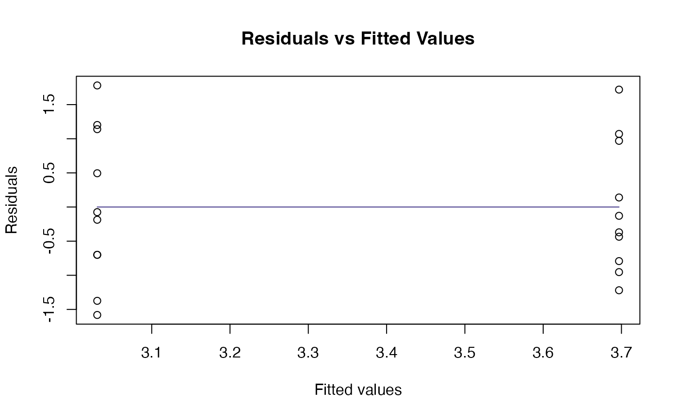

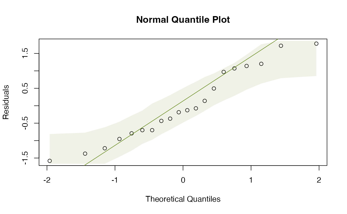
 by(guineapig$logErrors,guineapig$treatment,sd)
#> guineapig$treatment: C
#> [1] 0.521912
#> ------------------------------------------------------------ 
#> guineapig$treatment: N
#> [1] 0.445521

We are doing much better with assumptions: plots look better, standard deviations are more similar. Results became slightly more significant, which is not unexpected, as data are closer to normal (which usually means that tests based on linear models have more power).

Notice that there is no noticeable smoother or envelope on the residual vs fits plot – that is because for a t-test (and later on, one-way or factorial ANOVA designs) the mean of the residuals is exactly zero for all fitted values. Trying to assess the trend on this plot for non-linearity is not really useful, the only thing to worry about here is a fan shape. This would also show up on a smoother through the scale-location plot as an increasing trend:

 plotenvelope(ft_logGuineapigs,which=3)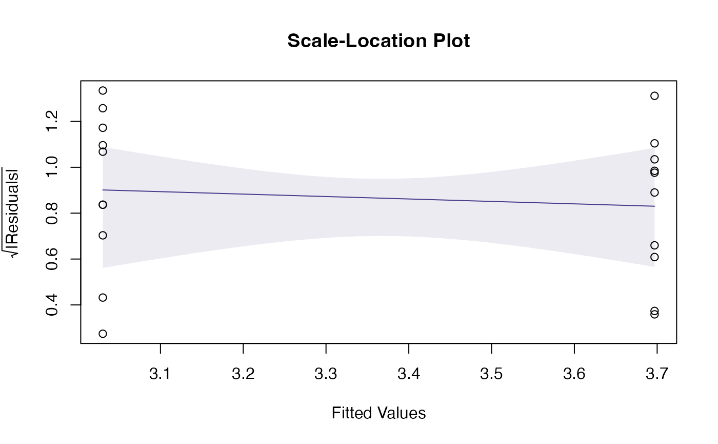

but there is no increasing trend so we are all good :)

Exercise 2.7: Influential value in the water quality data

 data(waterQuality)
 ft_water = lm(quality~logCatchment,data=waterQuality)
 summary(ft_water)
#> 
#> Call:
#> lm(formula = quality ~ logCatchment, data = waterQuality)
#> 
#> Residuals:
#>    Min     1Q Median     3Q    Max 
#> -7.891 -3.354 -1.406  4.102 11.588 
#> 
#> Coefficients:
#>              Estimate Std. Error t value Pr(>|t|)    
#> (Intercept)    74.266      7.071  10.502 1.38e-08 ***
#> logCatchment  -11.042      1.780  -6.204 1.26e-05 ***
#> ---
#> Signif. codes:  0 '***' 0.001 '**' 0.01 '*' 0.05 '.' 0.1 ' ' 1
#> 
#> Residual standard error: 5.397 on 16 degrees of freedom
#> Multiple R-squared:  0.7064, Adjusted R-squared:  0.688 
#> F-statistic: 38.49 on 1 and 16 DF,  p-value: 1.263e-05
 ft_water2 = lm(quality~logCatchment,data=waterQuality, subset=waterQuality$logCatchment>2)
 summary(ft_water2)
#> 
#> Call:
#> lm(formula = quality ~ logCatchment, data = waterQuality, subset = waterQuality$logCatchment > 
#>     2)
#> 
#> Residuals:
#>     Min      1Q  Median      3Q     Max 
#> -7.8709 -3.3107 -0.3438  4.5358 11.1955 
#> 
#> Coefficients:
#>              Estimate Std. Error t value Pr(>|t|)    
#> (Intercept)     77.71       9.70   8.011 8.46e-07 ***
#> logCatchment   -11.87       2.39  -4.966 0.000169 ***
#> ---
#> Signif. codes:  0 '***' 0.001 '**' 0.01 '*' 0.05 '.' 0.1 ' ' 1
#> 
#> Residual standard error: 5.522 on 15 degrees of freedom
#> Multiple R-squared:  0.6218, Adjusted R-squared:  0.5966 
#> F-statistic: 24.66 on 1 and 15 DF,  p-value: 0.0001691

The \(R^2\) value decreased a fair bit, which makes a bit of sense because we have removed from the dataset a point which has an extreme \(X\) value. \(R^2\) is a function of the sampling design and sampling a broader range of catchment areas would increase \(R^2\), and we have just decreased the range of catchment areas being included in analysis.

The \(P\)-value decreased slightly for similar reasons.

David Warton

2022-07-28