Chapter 1 -- 'STATS 101' Revision -- Exercise solutions and Code Boxes
David Warton
2022-07-28
Chapter1Solutions.RmdExercise 1.1: Experimental design issues
The issue is in the compare step – the mite treatment differed from the no mite treatment not just in presence or absence of mites, but also in presence or absence of crumpled up old leaves at the base of the plant. Crumpled up leaves could be beneficial to plants, e.g. by providing extra nutrients, or as a mulch that keeps moisture in the soil for longer.
The issue is in the replicate step – Beryl did not replicate the application of the treatment of interest. The oven temperature treatment was only applied once to each of 10 loaves. This means that she is unable to make generalisations about the effect of oven temperature because other aspects of the way treatment were applied in this one instance could also affect results, e.g. maybe the ovens were different (in size, shaoe, maybe one has a faulty door that leaks air out), maybe loaves were taken out slightly earlier for one batch than the another, maybe one oven was pre-heated better than the other. By replicating the baking process, with randomly chosen choices of treatment, these uncontrolled sources of variation can be considered as random and inferences can account for these.
The issue is in the randomise step – while teachers were instructed to ensure there wasn’t an undue proportion of well fed or undernourished children in either group, the point is that they were given responsibility for assigning students to treatments rather than this being done randomly. The weight difference at the start of the study suggests that some teachers did actually assign smaller and potentially undernourished children to the group receiving milk, presumably on compassionate grounds. This may or may not have been done consciously. Because the treatment groups were not homogeneous at the start of the study, it is not possible to conclude that changes during the study were due to milk – the groups were different to start off with so differences at the end of the study could be related to this. For example, it is possible that students receiving milk were smaller initially because they were later having a growth spurt, and so they grew more during the study for developmental reasons unrelated to milk.
Exercise 1.2: Which plot for which research question?
Plot (c), the boxplot of after-before differences, is best for looking at whether counts are larger after the gunshot than before. (If they are larger after, counts should be above zero.)
Plot (a), a scatterplot of after vs before counts, is best for studying of counts after the gunshot are relatd to counts before the gunshot sound.
Plot (b), a Tukey mean-difference plot of after-before differences against average counts, is best for looking at whether or not these counts measure the same thing. If After and Before counts are measuring the same underlying quantity, the differences should all be centered around zero, relatively close to it, and ideally they should not be a function of mean count.
Exercise 1.3: Raven count data – what data properties?
# ravens is a discrete, quantitative variable.
Sampling time is a categorical variable. Strictly speaking it is nominal but there are only two levels of sampling so ordering is irrelevant.
Exercise 1.4: Gender ratios in bats
There is one variable, bat gender. This is a categorical variable.
The research question is She would like to know if there is evidence of gender bias. If she is looking for evidence of gender bias then Kerryn is making inference about the true proportion of females in the colony, and she wants to know if it is different from a 50:50 ratio. So she wants to do a hypothesis test (of whether there is evidence that the true proportion of females is not 50%).
The specific procedure to use here is a one-sample test of proportions, e.g. using the ‘prop.test’ function on ‘R’:
prop.test(65,65+44)
#>
#>  1-sample proportions test with continuity correction
#>
#> data:  65 out of 65 + 44, null probability 0.5
#> X-squared = 3.6697, df = 1, p-value = 0.05541
#> alternative hypothesis: true p is not equal to 0.5
#> 95 percent confidence interval:
#>  0.4978787 0.6879023
#> sample estimates:
#>         p
#> 0.5963303
So there is marginal evidence that the true proportion of females in the colony is larger than 50:50 (since P is close to 0.05).
An appropriate graph here would be a bar graph

Exercise 1.5: Ravens and gunshots
As in Exercise 1.3, we have two variables:
- # ravens which is a discrete, quantitative variable.
- Sampling time which is a categorical variable taking two levels (before and after).
(You could argue that location is also a variable, it is categorical, and will be used to analyse the data using a linear model in Chapter 4.)
The question is whether ravens fly towards the sound of gunshots. This is not really a descriptive question because we want to know if ravens fly towards the sound of gunshots in general, not just at these 12 sites. This could best be approached using a hypothesis test, to test for evidence that ravens fly towards the sound of gunshots, but you could also construct a confidence interval for difference in counts, to estimate the size of the after-before mean count (with particular interest in whether it covers zero). Like this:
library(ecostats)
#> Loading required package: mvabund
data(ravens)
ravens1 = ravens[ravens$treatment==1,] #limit to just gunshot treatment
t.test(ravens1$Before,ravens1$After,paired=TRUE,alternative = "less")
#>
#>  Paired t-test
#>
#> data:  ravens1$Before and ravens1$After
#> t = -2.6, df = 11, p-value = 0.01235
#> alternative hypothesis: true mean difference is less than 0
#> 95 percent confidence interval:
#>       -Inf -0.335048
#> sample estimates:
#> mean difference
#>       -1.083333
So there is some evidence, although it is still a bit marginal, that ravens fly towards gunshot sounds (P is a bit above 0.01).
A suitable graph, as before, is a boxplot of the paired differences:
boxplot(ravens1$delta,ylab="After-Before differences")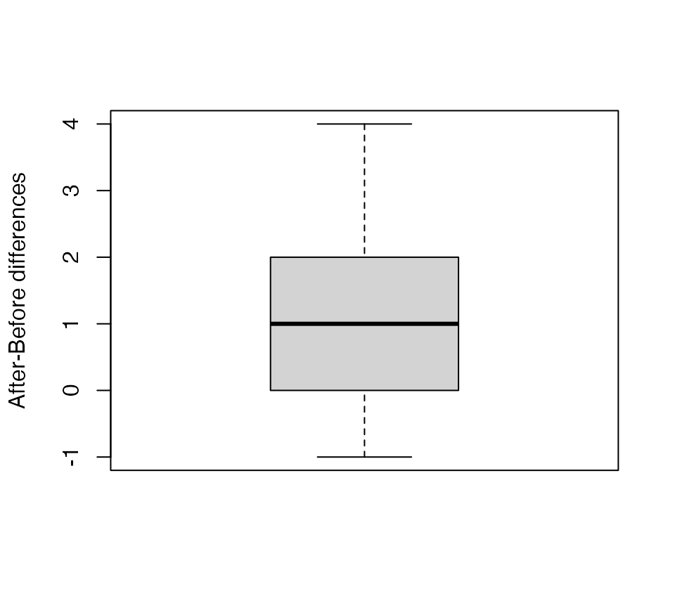
Exercise 1.6: Pregnancy and smoking
There are two variables:
-
errorsis quantitative -
treatmentis categorical with two levels (control and nicotine treatment)
The research question is what is the effect of a mother’s smoking during pregnancy on the resulting offspring?. In the context of this experiment, this means estimating the size of the change in average #errors in treatment vs control. So this is an estimation problem, we can use confidence intervals for average difference.
I would use a t-test procedure but put the focus on confidence interval estimation:
t.test(errors~treatment,data=guineapig, var.equal=TRUE)
#>
#>  Two Sample t-test
#>
#> data:  errors by treatment
#> t = -2.671, df = 18, p-value = 0.01558
#> alternative hypothesis: true difference in means between group C and group N is not equal to 0
#> 95 percent confidence interval:
#>  -37.339333  -4.460667
#> sample estimates:
#> mean in group C mean in group N
#>            23.4            44.3
So we are pretty sure (95% confident) that the true mean #errors made under nicotine treatment is between 4 and 37 more than in control.
I would use comparative boxplots:
plot(errors~treatment,data=guineapig)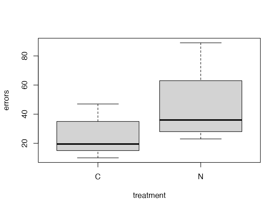
Exercise 1.7: Inference notation – Gender ratio in bats
\(n=65+44=109\).
This is \(\hat{p}\).
The true proportion of female bats in the colony is written as \(p\).
Exercise 1.8: Inference notation – raven counts
We know the value of \(\bar{x}_\text{after}-\bar{x}_\text{before}\).
We want to make inferences about the unknown value of \(\mu_\text{after}-\mu_\text{before}\).
Code Box 1.1: Analysing Kerry’s sex ratio data on bats
prop.test(65,109,0.5)
#>
#>  1-sample proportions test with continuity correction
#>
#> data:  65 out of 109, null probability 0.5
#> X-squared = 3.6697, df = 1, p-value = 0.05541
#> alternative hypothesis: true p is not equal to 0.5
#> 95 percent confidence interval:
#>  0.4978787 0.6879023
#> sample estimates:
#>         p
#> 0.5963303
2*pbinom(64,109,0.5,lower.tail=FALSE)
#> [1] 0.05490882
Exercise 1.9: Assumptions – Gender ratio in bats
If bats are randomly sampled from the colony, taking a simple random sample, then this assumption is satisfied.
Exercise 1.10: Assumptions – Raven example
There is no evidence of violation of the normality assumption (the points are all well within the envelope, with no particular trend).
Code Box 1.2: Normal quantile plot for the raven data
par(mfrow=c(1,2), mgp=c(1.75,0.75,0), mar=c(3,3,1,1))
Before = c(0, 0, 0, 0, 0, 2, 1, 0, 0, 3, 5, 0)
After = c(2, 1, 4, 1, 0, 5, 0, 1, 0, 3, 5, 2)
qqnorm(After-Before, main="")
qqline(After-Before,col="red")
library(ecostats)
qqenvelope(After-Before)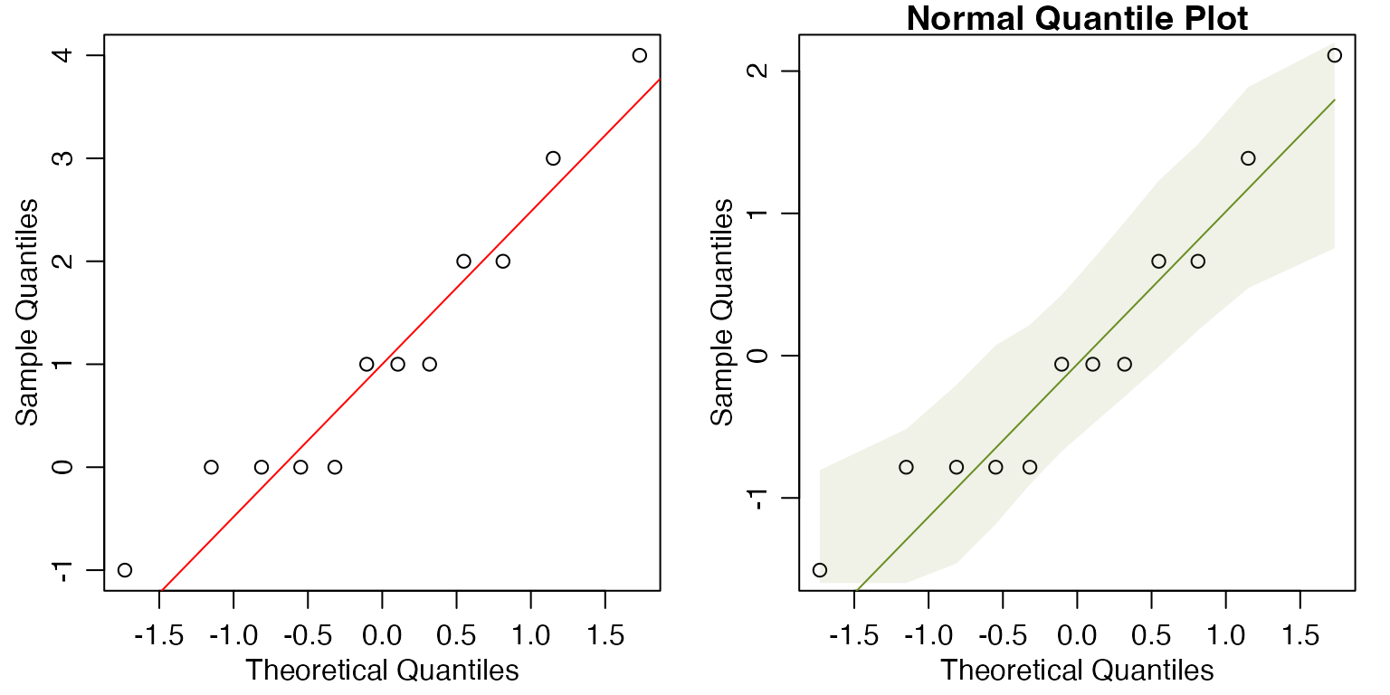
Code Box 1.3: log(y + 1)-transformation of the raven data
# Enter the data
Before = c(0, 0, 0, 0, 0, 2, 1, 0, 0, 3, 5, 0)
After = c(2, 1, 4, 1, 0, 5, 0, 1, 0, 3, 5, 2)
# Transform the data using y_new = log(y+1):
logBefore = log(Before+1)
logAfter = log(After+1)
# Construct a normal quantile plot of the transformed data
qqenvelope(logAfter-logBefore)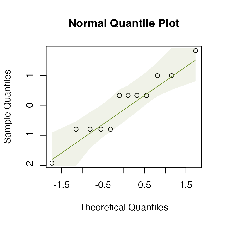
Exercise 1.11: Height and latitude
Angela is interested in (interval) estimation – to understand how height is related to latitude.
There are two variables:
-
heightis quantitative -
latitudeis quantitative
Exercise 1.12: Transform plant height?
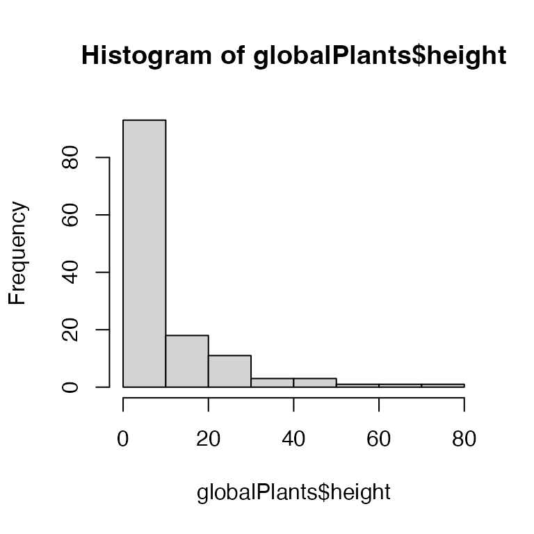
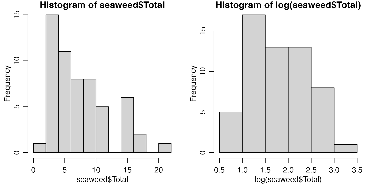
The data are bunched up against zero – plants cannot have negative height! A log-transformation might be worth a try
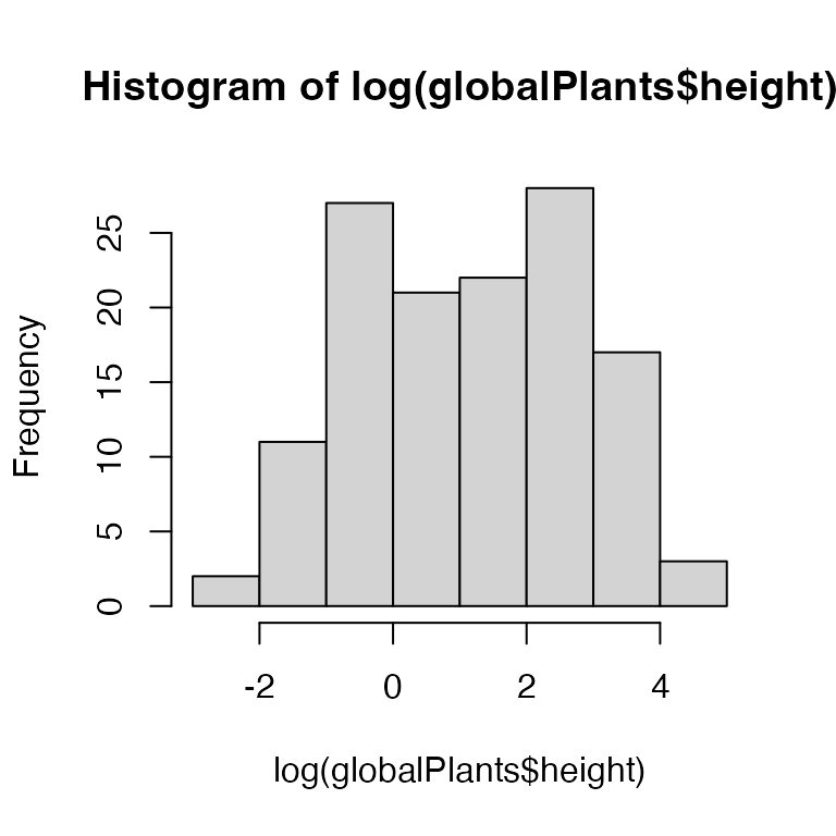
This has removed the boundary and seems to have removed the strong right-skew.
Exercise 1.13: Snails on seaweed
The research question is Does invertebrate density change with isolation? meaning that we have a specific hypothesis of interest (no change) and we are looking for evidence against this hypothesis. So a hypothesis test is appropriate here.
There are two variables:
- invertebrate density is quantitative and is the response variable of interest.
- isolation is an experimental factor taking three levels (0, 2 or 10 metres)
I would use comparative boxplots, like this:
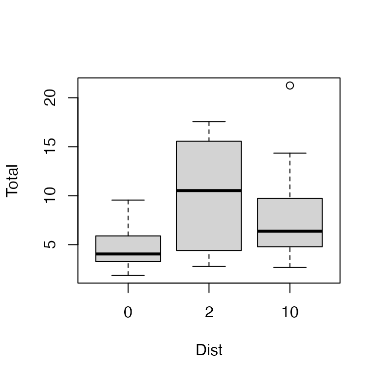
I used boxplot instead of using plot
because Dist is currently a numerical variable rather than
a factor, so the default behaviour of plot would have been
to do a scatterplot :(
